House Prices from Magazines, Realtors, and the Land Registry

(1)

BIS Papers

No 64

Property markets and

financial stability

Proceedings of a joint workshop organised by the BIS and the Monetary Authority of Singapore in Singapore on 5 September 2011

Monetary and Economic Department

March 2012

JEL classification: E30, E44, E58, R21, R31.

Keywords: house prices, housing credit, credit conditions, monetary policy, macroprudential regulation

(2)

Papers and discussant remarks in this volume were prepared for a workshop organised by the BIS and the Monetary Authority of Singapore (MAS) in Singapore on 5 September 2011. The views expressed are those of the authors and do not necessarily reflect the views of the BIS or the institutions/central banks represented at the meeting. Individual papers (or excerpts thereof) may be reproduced or translated with the authorisation of the authors concerned.

This publication is available on the BIS website (www.bis.org).

ISSN 1609-0381 (print) ISBN 92-9131-107-3 (print) ISSN 1682 7651 (online) ISBN 92-9197-107-3 (online)

(3)

Foreword

The Bank for International Settlements (BIS) and the Monetary Authority of Singapore (MAS) jointly organised a workshop on property markets and financial stability in Singapore on 5 September 2011. The workshop aimed to bring together academics and researchers at central banks, regulatory agencies and international organisations to present and discuss ongoing theoretical and empirical work in the field. In response to their call for papers, the organisers received 67 submissions from central banks, public agencies, international organisations and academic institutions. From these, a paper selection committee comprising staff of the BIS, the MAS and academia chose seven papers organised around the following four themes: (1) lessons from the crisis; (2) house price assessment; (3) housing booms and busts; and (4) property, credit and markets.

All in all, 39 participants took part, including central bank economists as well as academics from Asia and the Pacific, Europe and the United States. Assistant Managing Director Andrew Khoo of the MAS and Frank Packer, Head of Financial Stability and Markets for Asia and the Pacific of the BIS, delivered the opening remarks. Professor Timothy Riddiough at the University of Wisconsin gave a keynote speech. This volume is a collection of the opening remarks, the keynote speech, revised versions of all the papers presented during the workshop, as well as discussant remarks on these papers.

(4)

(5)

Programme

08:45–09:00 Welcome remarks

Andrew Khoo, Assistant Managing Director, Monetary Authority of Singapore

Frank Packer, Head of Financial Stability and Markets for Asia and the Pacific, BIS

Chair: Wong Nai Seng (MAS)

09:00–09:45 Keynote speech by Timothy Riddiough (University of Wisconsin)

“The first subprime mortgage crisis and its aftermath”

Session 1 Lessons from the crisis

09:45–10:30 “Commercial real estate loan performance at failed US banks” Andrew Felton (FDIC) and Joseph B Nichols (Federal Reserve Board)

Discussant: Ilhyock Shim (BIS) 10:30–11:00 Group photo and coffee break

Session 2 House price assessment

Chair: Kenneth Kuttner (Williams College)

11:00–11:45 “House prices at different stages of the buying/selling process” Chihiro Shimizu (Reitaku University), Kiyohiko Nishimura (Bank of Japan) and Tsutomu Watanabe (Hitotsubashi University and University of Tokyo)

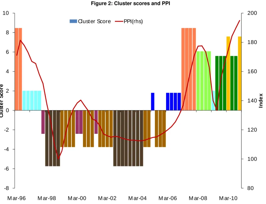
Discussant: Deng Yongheng (National University of Singapore) 11:45–12:30 “A cluster analysis approach to examining Singapore’s property

market”

Lily Chan, Ng Heng Tiong and Rishi Ramchand (MAS)

Discussant: Phang Sock Yong (Singapore Management University) 12:30–14:00 Lunch

Session 3 Housing booms and busts

Chair: Deng Yongheng (National University of Singapore) 14:00–14:45 “Dealing with real estate booms and busts”

Christopher Crowe, Giovanni Dell’Ariccia, Deniz Igan and Pau Rabanal (IMF)

Discussant: Veronica Warnock (University of Virginia)

(6)

Session 3 (cont) Housing booms and busts

14:45–15:30 “Capital inflows, financial innovation and housing booms”

Filipa Sá (University of Cambridge), Pascal Towbin (Bank of France) and Tomasz Wieladek (Bank of England)

Discussant: Kenneth Kuttner (Williams College)

15:30–16:00 Coffee break

Session 4 Property, credit and markets

Chair: Eli Remolona (BIS)

16:00–16:45 “Credit standards and the bubble in US house prices: new econometric evidence”

John V Duca (Federal Reserve Bank of Dallas), John Muellbauer (University of Oxford) and Anthony Murphy (Federal Reserve Bank of Dallas)

Discussant: Frank Warnock (University of Virginia)

16:45–17:30 “Credit conditions and the real economy: the elephant in the room” John Muellbauer and David M Williams (University of Oxford) Discussant: Chris Thompson (Reserve Bank of Australia)

17:30–18:15 Panel discussion

Moderator: Timothy Riddiough (University of Wisconsin) Panellists: Wong Nai Seng (MAS)

Frank Packer (BIS)

Frank Warnock (University of Virginia)

(7)

List of participants

Central banks

Australia Reserve Bank of Australia Chris Thompson

Deputy Head, Financial Stability Department

China People’s Bank of China

Liu Zhenhua

Deputy Research Director, General Executive Office

France Bank of France

Pascal Towbin Economist

Hong Kong SAR Hong Kong Monetary Authority Eric Kan

Senior Manager, Banking Supervision Department Matthew Yiu

Senior Manager, Research Department

India Reserve Bank of India

Venkata Raman Sankaran

Assistant General Manager, Department of Banking Operations and Development

Indonesia Bank Indonesia

Dwityapoetra S Besar

Research Executive, Banking Research and Regulation Department

Japan Bank of Japan

Hiroaki Kuwahara

Deputy Head, International Department

Korea Bank of Korea

Yong-Sun Kim

Head, Financial Stability Analysis Team Malaysia Central Bank of Malaysia

Hamim Syahrum Ahmad Mokhtar

Deputy Director, Financial Surveillance Department

Netherlands Netherlands Bank

Jan Marc Berk

Division Director, Statistics and Information Department Philippines Bangko Sentral ng Pilipinas

Josephine D Abdulrahman

Bank Officer IV, Office of MD-Supervision and Examination Subsector III

Amabelle D Garcia

Bank Officer III, Office of Supervisory Policy Development

(8)

Singapore Monetary Authority of Singapore Andrew Khoo

Assistant Managing Director Wong Nai Seng

Executive Director, Macroeconomic Surveillance John Sequeira

Principal Economist, Economic Analysis Ng Chuin Hwei

Director, Prudential Policy Lily Chan

Lead Economist, Macroeconomic Surveillance Ng Heng Tiong

Lead Economist, Macroeconomic Surveillance Rishi Ramchand

Senior Economist, Macroeconomic Surveillance

Sweden Sveriges Riksbank

Albina Soultanaeva

Senior Economist, Financial Stability Department

Thailand Bank of Thailand

Buncha Manoonkunchai

Senior Expert, Financial Institution Strategy United States Federal Reserve Board

Joseph B Nichols Economist

Federal Reserve Bank of Dallas John V Duca

Vice President and Senior Policy Advisor

Regulatory agencies

China China Banking Regulatory Commission Zhang Xiaopu

Deputy Director-General

Academic institutions and international organisations

IMF International Monetary Fund

Mangal Goswami

Deputy Director, IMF-Singapore Regional Training Institute (STI)

Shinichi Nakabayashi

International Consultant Economist, IMF-STI Deniz Igan

Economist

Japan Hitotsubashi University and University of Tokyo Tsutomu Watanabe

Professor

(9)

Singapore National University of Singapore Deng Yongheng

Professor

Singapore Management University Phang Sock Yong

Professor

United Kingdom University of Oxford David Williams

Post-doctoral Researcher, Department of Economics United States University of Virginia’s Darden School of Business

Frank Warnock Professor

Veronica Warnock Senior Lecturer

University of Wisconsin-Madison Timothy Riddiough

Professor

Williams College

Kenneth Kuttner Professor

Bank for International Settlements

Eli Remolona Chief Representative

Frank Packer

Head of Financial Markets and Stability for Asia and the Pacific Ilhyock Shim

Senior Economist

(10)

(11)

Welcome remarks

Andrew Khoo¹

Overview and background

Professor Timothy Riddiough, colleagues from the BIS, IMF, central banks, regulatory agencies and academia, ladies and gentlemen. Good morning.

Welcome to this workshop. We received more than 60 papers from many countries, with submissions from central banks, public agencies, supranational organisations, and academic institutions. I would like to thank everyone for their support. The very good response reflects the strong interest in this growing and important area of research.

Property market volatility poses financial stability challenges

The theme of this workshop is property markets and financial stability. Maintaining stability in property markets has been challenging for authorities across Asia in the last few years. Between 2005 and 2008, property prices in Asian economies rose rapidly. This reversed during the Global Financial Crisis, as the downturn affected incomes, confidence and the availability of financing. However, as the Asian economies rebounded, so did property prices, reaching record levels in a number of countries.

Property markets are prone to cycles, in part because supply is inelastic in the short term. This cyclical behaviour is exacerbated by several factors.

First, property is both a consumption good and an investment good. While rising prices would normally mean lower consumption, expectations of further price increases could induce more investment demand. Price momentum may escalate as valuations are usually set with reference to the latest transacted prices.

Second, housing markets tend to be highly leveraged. Most homebuyers borrow to finance their purchases, sometimes up to 80% or 90% of the value of the property. And because mortgage loans are collateralised and have historically low default rates, banks are prepared to lend at high loan-to-value ratios. In a rising market, banks are willing to lend more as the value of the collateral increases. Easier credit may contribute to further increases in house prices. But this feedback loop quickly reverses when prices are falling. Lenders tighten underwriting standards. Existing housing loans with small equity buffers may slip into negative equity and some borrowers may be forced to sell. This puts further downward pressure on prices.

Third, housing generally accounts for a significant proportion of households’ balance sheets and banks’ loan portfolios. In Singapore, property forms almost 50% of household assets while housing loans account for three quarters of total household debt. They also make up about 17% of bank lending to non-bank borrowers. As a result, adverse developments in housing markets can have a material impact on household wealth and the health of the banking system. This could then dampen household demand and banks’ ability to supply credit, and in turn economic growth. Further, construction accounts for as much as 10% of

1 Assistant Managing Director, Monetary Authority of Singapore.

(14)

output in some Asian economies and could pose a significant drag on growth should activity in the sector falter. Indeed, the United States, Ireland and Spain are recent examples of how property sector imbalances could cause issues as households and banks delever.

The challenge of maintaining stability

Therefore, stable property markets matter to households, to the financial system and to the economy. Asia’s policy responses to property market developments over the last few years reflect this awareness. Besides encouraging individuals to borrow and banks to lend prudently, policy measures sought to mitigate the build-up of system-wide leverage. These so-called macroprudential tools are not new, as some Asian authorities have been using them since the 1990s. But there has been greater interest in such measures following the crisis.

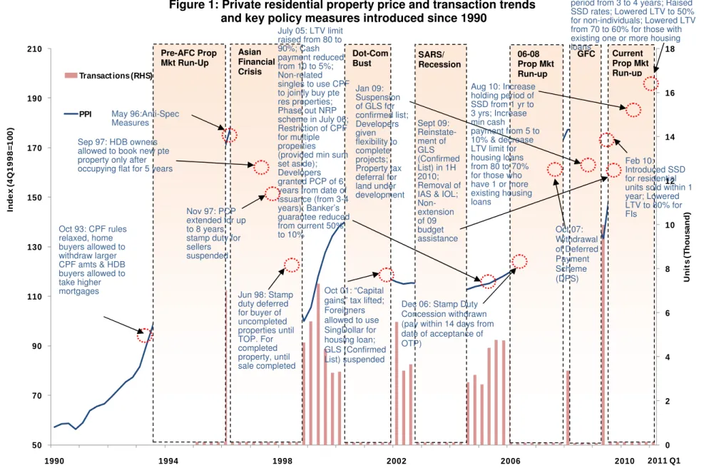
In Singapore, the government disallowed certain loan schemes that may have encouraged property speculation, introduced a seller stamp duty, lowered LTV ratios and raised the minimum cash payment required for property purchases. Public housing construction has gathered pace and more land has been made available for private housing development. The measures have to some extent moderated the market, with the rate of increase in private property prices slowing in each of the last seven quarters. Transaction activity has fallen as well.

Our approach has been, from a whole-of-government perspective, targeted and incremental. Measures were focused on discouraging short-term speculative activity that could distort underlying prices, whilst encouraging greater financial prudence among property purchasers. Policies were fine-tuned over time to take into account implementation experience and market impact.

Research agenda

Policymakers need to deepen their understanding of the range of macroprudential tools and their efficacy. Unlike in monetary policy, where there are more established models of policy targets, transmission mechanisms and policy reaction functions, research on macroprudential tools is still at an early stage.

More research needs to be done on property markets and their interactions with the financial system and the real economy. The use of macroprudential tools in Asia and elsewhere to deal with property market pressures offers an opportunity to evaluate the effectiveness of these tools and consider how they can be refined. Policy design and implementation will benefit from a better understanding of market behaviour and interlinkages. Research findings can also feed into ongoing efforts by the IMF, the BIS and the FSB to develop guidance on issues such as the institutional set-up for macroprudential policy, tools for risk monitoring and assessment, and the design, timing and communication of policy measures. Workshops like this provide a useful forum in which to make progress on establishing a robust framework for macroprudential policies.

Conclusion

Before I end, I would like to thank the BIS for its partnership in organising this conference. On behalf of the organisers, I would like to express our appreciation to Professor Timothy Riddiough, our keynote speaker, and to Kenneth Kuttner, Frank and Veronica Warnock,

(15)

Deng Yongheng, Phang Sock Yong and Chris Thompson for kindly agreeing to be chairpersons, discussants and members of the scientific panel.

I wish you all an engaging and fruitful conference.

(16)

(17)

Welcome remarks

Frank Packer¹

Allow me on behalf of the Asian Representative Office of the BIS also to welcome you all here. I also want to thank the Monetary Authority of Singapore (MAS) for being so receptive to our proposal nearly one year ago that we co-host this workshop on property markets and financial stability.

The BIS Asian Office was asked in 2010 by its Consultative Council of Asian central bank Governors (ACC) to focus a significant portion of its research work and the support it gives central banks over the next few years on the theme of property markets and financial stability in the region. We were asked to collaborate with ACC member central banks to design and implement research work.

There are four broad general areas that the Governors asked us to look at. First of all, how should authorities best monitor and assess valuations in housing markets? Important methodological issues include how to check the representativeness and completeness of sample transactions that underlie housing price indices, as well as how to account for the heterogeneity of the housing market.

The second topic covers housing finance arrangements and their market impact. In particular, we are interested in what institutional variables might contribute to unsustainable growth in mortgage markets. Might some types of housing finance systems be less prone to crisis?

A third category on our research agenda is the relationship between property markets and the health of the banking sector. Here we are particularly interested in the tendency of bank lending in the real estate sector to be procyclical.

Finally, the Governors have asked for work on the impact of various policy instruments on property prices and related transactions. This is a topic very close to the hearts of policymakers in Asia, where there is a very rich record of macroprudential policies.

This research workshop, which brings academic scholars together with central bank and financial supervisory experts, covers all of these topics and more.

A paper selection committee consisting of John Sequeira and Wong Nai Seng from the MAS, myself and Haibin Zhu of the BIS and scholars Frank Warnock and Yongheng Deng chose what we thought were the seven best papers from around 70 submissions. We were looking for papers that not only showed rigour and care in research, but were also relevant to policymakers and might provoke an active discussion. I think we’ve got an excellent line-up of papers and speakers, the fruits of which we will be enjoying over the next few days. I’d like to brief you all here a bit on the format of the workshop. The first day’s proceedings will consist of the presentation of a keynote address by Tim Riddiough, Professor at the University of Wisconsin-Madison and incoming President of the American Real Estate and Urban Economics Association, as well as the presentation and discussion of the selected research papers.

Tomorrow, there will be presentations by central banks and supervisors about current conjunctural developments in property markets as well as policy responses. The second

1 Head of Financial Stability and Markets for Asia and the Pacific, Bank for International Settlements.

(18)

day’s sessions will be in front of a somewhat smaller audience in the interest of confidentiality.

So without further ado, allow me to introduce the chair of Session 1 on the lessons of the financial crisis, Wong Nai Seng of the MAS. Nai Seng heads the Macroeconomic Surveillance Department of the MAS which is responsible for conducting research and surveillance and providing policy advice on financial stability issues. We are very lucky to have him here chairing the next session, and the floor is now his.

(19)

The first sub-prime mortgage crisis and its aftermath

Timothy J Riddiough¹

Introduction

Financial markets in the years and months leading up to the financial crisis of 2007–08 were characterised by growth in the shadow banking sector, pyramiding and hidden leverage in the consumer and financial sectors, off-balance sheet financing by systemically important firms, and mortgage securitisation and other “creative” financing schemes that some say resembled games of “hot potato” and “hide the sausage”. The failure of a prominent financial institution triggered an eventual full collapse in stock prices, resulting in, among other things, a foreclosure crisis with long-lasting negative spillovers into the real economy.

Many believe the recent crisis to be unprecedented, where, for example, Hyun Song Shin (2010) wrote: “The global financial crisis that erupted in the summer of 2007 has the distinction of being the first post-securitisation crisis in which banking and capital market developments have been clearly intertwined.” In this speech I will present research I am conducting on the US panic of 1857 that contradicts Professor Shin’s observation, where the 1857 panic bore eerie similarities to the more recent panic.²

The older panic, which occurred almost exactly 150 years prior to the more recent panic, had, in addition to the factors noted above, global capital flows emanating primarily from England and the Continent with clearly intertwined banking and capital markets. And, although sub-prime mortgage lending and securitisation were perhaps not as widespread as they were in the current crisis, they played a very central role in propagating the panic from a few strategically placed firms located near the frontier of the Old Northwest back east to New York City and Europe.³

It is said that every crisis is similar and that every crisis is different. Identification of the relevant similarities and differences requires memory and retained knowledge, where this knowledge can be gained and retained in different guises. The broader objective of this speech is to argue that historical perspective, and more generally inductive methods to research, provides a strong complement to more traditional deductive research methods such as large-sample econometric analysis.

This speech is organised in three acts. The first act sketches the background of the US economy in the years and months leading up to the crisis of 1857 (which occurred in late August and lasted through October of that year). The second act analyses the sub-prime mortgages and their securities that existed at the time, which were known as the railroad farm mortgage (RRFM) and the RRFM-backed security. The third and final act considers the failure of the prominent financial institution that triggered the panic, and the panic’s aftermath as it specifically related to the RRFMs and their securities.

1 University of Wisconsin – Madison.

2 This speech is derived directly from ongoing research I am jointly conducting with Howard Thompson on the panic of 1857 and its aftermath. See specifically Riddiough and Thompson (2011).

3 Much of the modern treatment of the panic of 1857 is from a macro-banking perspective. See, for example, Calomiris and Schweikart (1991). Older and more historically focused treatments of the crisis include Van Vleck (1943), Fishlow (1965), Huston (1987) and Stampp (1990). One of the most interesting and informative treatments of the crisis comes shortly after the crisis occurred, from Gibbons (1859).

(20)

Act I: The years and months leading up to the panic of (late August

through October) 1857

Some historical background on the 20 years leading up to the panic of 1857 is necessary to appreciate the panic’s many contributing factors. At a very basic and very real level, the panic of 1857 was the natural culmination of events that started with the even more severe panic of 1837.

For my story, there are two essential direct consequences of the earlier panic that are relevant. First, as a result of state-level funding of transportation infrastructure development (canals and the relatively new invention of the railroad), a number of states defaulted on their bonds after the panic of 1837. This experience caused many states to restrict any public funding of transportation projects. These restrictions shifted the burden of financing public goods to cities and more often individuals, resulting in a number of distorting effects. Second, bank failures in the 1837 panic were related to “money-run” as opposed to “deposit-run” problems, as deposit-based banking was in its infancy in the United States. Thus, the free banking era was born after 1837, with most of the regulatory focus on the quality of money printed by individual banks. Deposit-based banks consequently operated at the fringes of banking and bank regulation at the time, and were in effect shadow banks. By the time of the 1857 panic, other non-money issuing firms such as railroads also operated as shadow banks by intermediating between direct capital suppliers and indirect investors.

In addition to state-level funding of infrastructure projects, significant amounts of the capital channelled into investment prior to the 1837 panic came from England and the Continent. After that crash, foreign investors said, “Never again!” Time and a yearning for easy riches erode many things, however. One key event that prompted a change in attitude among foreign investors was the California gold strike and gold rush of 1848 and 1849. That event significantly added to the gold stock of the United States and the world, resulting in, among other things, increased credit availability, growth in world trade, industrial construction and railroad building (Van Vleck (1943, pp. 38–39)).

Shortly after the gold rush, a railroad boom indeed began in earnest, as newfound wealth and an influx of foreign capital made its way into the hands of railroads and their promoters. Figure 1 shows the extent of the boom, with the amount of investment and added railways from 1850 to 1856. It is estimated that in excess of 25 per cent of the US GDP derived from the railroads during the mid-1850s. As noted in Panel B of the figure, Ohio, Indiana, Illinois, Michigan, Wisconsin and Iowa were considered western states at the time, at or near the frontier of the country and of railroad development. Figure 2 provides a visual depiction of railroad investment/construction activity during the 1850s.

Largely because of the huge capital appetite of the railroads as a result of their stupendous growth during the 1850s, Wall Street began taking on its more modern character as an investment banker in addition to providing stock brokerage services and other methods of sourcing capital and making markets for securities. These developments helped lay the foundation for new creative ways to package securities for sale to investors.

The Crimean War raged in central Europe, lasting from late 1853 to early 1856. This war increased the demand for agricultural products grown and processed in the United States, where an increasing proportion of farming activity was migrating to the western states noted in Panel B of Figure 1. Huston (1983) and others have argued persuasively that the agricultural demand boom due to the Crimean War, followed by a decline in demand as the war approached its end, contributed to falling food commodity prices starting in 1855 and continuing through to the 1857 panic. Declining demand was coupled with a softening macroeconomy, particularly in the North, as well as ruthless and predatory competition among railroads in that most networked of industries. The result of this dynamic was railroad track being laid well ahead of demand, particularly in the frontier states of Illinois and Wisconsin.

(21)

Figure 1 Panel A: miles added and investment

index, 1850–1856

Panel B: railroad investment as percentage of GDP, and miles added in

Ohio, Indiana, Illinois, Michigan, Wisconsin and Iowa as percentage of total

miles added, 1848–1856

1,000 1,500 2,000 2,500 3,000 3,500

1850 1851 1852 1853 1854 1855 1856 Investment index

Miles added

5 15 25 35 45 55 65 75

1848 1849 1850 1851 1852 1853 1854 1855 1856 As a percentage of total miles added

As a percentage of GDP

Note: In Panel A, investment equals gross investment times 30, in 1860 dollars.

Sources: Figure from Wahl (2009, Figures 5 and 6). His sources are Wilson and Spencer (1950, p.339), Stover (1987, p.317), Fishlow (1965, Table 16), and Historical Statistics of the United States, Millennial Edition (www.hsus.cambridge.org).

Figure 2

Western railway construction

Source: Fishlow (1965, Map 2).

(22)

Softening demand for long-haul transport of foodstuffs and other products produced at or near the frontier, along with overcapacity due to railroad construction occurring ahead of demand, caused a sharp decline in railroad share prices during the mid-1850s. These declines, implying increases in the cost of equity capital for the railroads, could not have come at a worse time as the railroad investment boom was moving ahead at full steam (pun intended).

A reduction in the supply of equity capital and increases in its cost had three implications for the railroads. First, it caused them to use more debt relative to equity to finance themselves, resulting in higher-leveraged firms. Second, it had the effect of increasing the opacity of the railroads, making it harder for outsiders to ascertain their true financial condition.⁴ Third, it caused the railroads to become increasingly creative in the ways they sourced and packaged finance, with many railroads engaging in stock-watering schemes, off-balance sheet financings, and generally doing anything they could to raise capital but not disclose its true cost or its leveraging effects.

It was against this backdrop that the panic of 1857 occurred. Importantly, not unlike the more recent panic, there were a number of “mini-events” in the months leading up to the big event that shook the confidence of investors. Calomiris and Schweikart (1991) and Wahl (2009) stress the importance of the Dred Scott decision, which in early 1857 opened the far western American frontier to slavery. Its effects were to chill westward migration, land-value increases and railroad expansion. In early August, two prominent New England mills closed their doors due to declining demand, and at about the same time it was revealed that the Michigan Southern railroad had engaged in a Ponzi-like stock-watering scheme.

Finally, on 24 August 1857, the Ohio Life Insurance & Trust Company (OLITC) failed, triggering a full-scale meltdown in the markets. Railroad share prices plunged in the week following the failure, where, as shown in Table 1 and Figure 3, western railroads took a disproportionate share of the punishment. The four railroads singled out as “Other Western Railroads” in Table 1 experienced precipitous declines in share prices. The first two firms received most of the recent financing from the OLITC, as OLITC gambled on resurrection by doubling down its bets on the struggling railroads. The other two firms were laying track right at the north-western frontier of the country, in Wisconsin. These firms figure prominently in the next act of this speech as two of the biggest sub-prime mortgage lenders in the country.

4 George Hudson, the king of British railroads in the 1840s, famously said, “I will have no statistics on my railroads”. His counterparts a decade later in the United States had similar sentiments. Chancellor (1990), in his entertaining book on the history of financial speculation, notes of Hudson: “His false accounting and generous dividends had misled speculators into believing the railroads were more profitable than they actually were.”

(23)

Table 1

Stock price changes of railroads, grouped by region,

immediately prior to and immediately after the date OLITC announced failure Railroad %_{ stock}

price ART data week prior

%_{ stock} price ART data

week of

%_{ stock} price NYT-BA data

week prior

day after

week of New England RRs

Boston & Lowell 0.00 0.00 N/A N/A N/A

Boston & Prov 2.70 -1.32 N/A N/A N/A

Boston & Worcester 0.00 0.00 N/A N/A N/A

Eastern of Mass. 0.00 0.00 N/A N/A N/A

Western of Mass. 0.00 0.00 N/A N/A N/A

Regional average 0.56 -0.28 N/A N/A N/A

Middle States RRs

Baltimore & Ohio 0.00 5.26 N/A N/A N/A

New York Central -2.50 2.56 -2.54 -3.58 -3.58

New York & Erie -9.68 -28.57 -8.80 -17.25 -21.05

Penn Central 0.00 -8.60 N/A N/A N/A

Regional average -1.92 -4.30 N/A N/A N/A

Western RRs Chicago Burl. &

Quincy ^0.00-33.33 N/A N/A N/A

Cleveland & Toledo -2.13 -13.04 -10.57 -7.78 -8.36

Illinois Central -6.67 -28.57 -2.82 -7.14 -20.54

Michigan Central -7.23 -22.08 -6.97 -2.28 -12.38

Other Western RRs Cleveland &

Pittsburgh

-16.67 -60.00 N/A N/A N/A

Marietta & Cincinnati _0.00-60.00 N/A N/A N/A

La Crosse &

Milwaukee -21.21 -80.77 -31.20 -6.98 -51.16

Milwaukee &

Mississippi -11.11 -58.33 -2.04 -12.50 -25.00

Source: “United States railway share and bond list,” American Railway Times, New York Times, and Boston Advertizer.

(24)

Figure 3

Railroad stock indices, 1 March 1857–10 October 1857

Source: From Wahl (2009, Figure 14). His source is Sylla et al (2002).

Act II: Necessity as the mother of invention

As mentioned earlier, railroads at the north-western frontier were laying track ahead of demand. This was particularly true in Wisconsin, which was recognised as being endowed with extremely fertile land but having little in the way of financial capital or infrastructure outside the city of Milwaukee.

Given the speculative nature of railroad investment at the frontier, coupled with the huge capital demands of the railroad business, it is no surprise that funding such ventures proved daunting along several dimensions. First, the conventional wisdom at the time was that anything in excess of a 50 per cent leverage ratio for a railroad was imprudent.⁵ This forced railroads to source significant amounts of equity capital to finance investment. Most of the available equity capital resided on the north-eastern seaboard of the United States and in Europe. This capital, in turn, wanted to see a slug of local equity capital invested as a signal of the quality of the railroad. With no local equity capital, there was therefore no arm’s-length equity and hence there were strict limits on the ability to debt-finance, all of which implied no new investment. Second, as also noted earlier, many north-western states, Wisconsin included, had amended their constitutions to restrict the public financing of transportation infrastructure projects. This consequently excluded a very important potential source of local finance, forcing the railroads to become even more promotional and creative than they already were.

5 Henry Varnum Poor was the most ardent and articulate spokesperson in this regard. See Chandler (1956) for a warm and well-executed biography of Poor and his times.

(25)

Wisconsin outside of Milwaukee was land rich but “as poor as poverty’s grandmother”. The question then was how to source the necessary local equity capital that would open the floodgates for even more debt and equity capital flowing from the east. In the early 1850s the owners of the La Crosse & Milwaukee railroad hit on an idea. Why not approach local farmers, particularly those farmers whose property lay near the path of the railroad line and its depots, and ask them to mortgage their farm to the railroad in return for shares of stock in the railroad? The dividends from the stock would be at least equal to the interest required on the mortgage, where the dividend-interest swap negated any need for the farmer to come out of pocket for interest payments on the debt. In fact, no cash changed hands at all between the farmer and the railroad in this debt-for-equity swap.

From the farmer’s perspective, it was a beautiful transaction. At no apparent cost, the farmer increased the value of his land by aiding in the laying of track near his property. He also got to share in the success of the railroad through appreciation in the stock price. There was no down payment required on the mortgage. There was also no loan documentation required – only an appraisal done by an agent of the railroad. The allowable loan-to-value ratio on the mortgage was 67 per cent – significantly higher than the prudent accepted maximum loan-to- value ratio at the time of 50 per cent. These mortgages were in essence sub-prime loans. They were even better than the sub-prime loans offered during the recent crisis, in that the railroad farm mortgages were high-leverage, no-documentation, no-down-payment loans that in fact required no mortgage payment whatsoever.

This brilliant conception accomplished several objectives at the same time for the railroad. By issuing shares to acquire an asset – the railroad farm mortgage – the railroad could claim that it successfully sourced local equity capital. The thorny issue of consideration – ie taking a mortgage in lieu of cash to fund the purchase price of the stock – could be addressed in a second step. The transaction also reduced the reported leverage of the railroad, since 100 per cent equity had been issued to finance ownership of the RRFMs. Figure 4 displays a stylised balance sheet of a railroad that starts with assets of 100 and a 50 per cent leverage ratio. The all-equity-financed purchase of 100 of the RRFMs is seen to double the size of the company and reduce the leverage ratio by half.

Figure 4

Stylised balance sheet statements of railroad with railroad farm mortgage purchases

Panel A: Prior to RRFM financing

Assets Liabilities RR Assets 100 Debt 50

Equity 50 Reported leverage ratio: 50 per cent.

Panel B: After RRFM financing

RRFM 100 Equity 150 Reported leverage ratio: 25 per cent. Source: Riddiough and Thompson (2011).

(26)

Figure 5

Partial prospectus of a farm mortgage bond financing from 1856

Now, the second step of the transaction was for the railroad to monetise the RRFMs so that it could purchase the track and equipment necessary to expand the line. The solution to this problem resulted in what we believe to be the first case of mortgage securitisation executed in the United States. It was a railroad farm mortgage-backed security – effectively a covered

(27)

bond offered by the railroad to potential investors located on the east coast and in Europe. Figure 5 displays the first four pages of an 1856 offering of farm mortgage bonds by the Racine & Mississippi railroad, which we believe is representative of other offerings that occurred at the time.⁶ As seen in the offering, three sources of security are offered to the investor: i) the note, which states the financial obligation of the farmer to repay the stated mortgage amount; ii) the mortgage, which offers the farm as collateral; and iii) the bond of the railroad, which offers its reputation for repayment and its other assets on an unsecured basis.

Notice, however, that there is no mention of the fact that the farmer pays no interest on the underlying mortgage collateral. Also notice that no other documentation is offered on the mortgage loans, other than assurances that a loan-to-value ratio of 67 per cent is not exceeded based on an appraisal done by an agent of the railroad.

These frontier railroads were successful in their RRFM-backed securities offerings, generally raising 80 cents on the face value dollar with a coupon interest rate of 10 per cent. Figure 6 references and extends the stylised balance sheet seen in Figure 4 by showing what happens when RRFMs are securitised and sold to investors, with proceeds used to invest in railroad track and equipment. Issuance proceeds of 80 are recorded as railroad assets, while the discount of 20 on the securities (following the practice of the day) was capitalised and carried as an asset by the railroad. The contingent covered bond liability is “off-balance sheet” and hence ignored, with the leverage ratio remaining at 25 per cent. What a beautiful transaction, not only for the farmer, but also for the railroad!

Figure 6

Stylised balance sheet statements of railroad with

railroad farm mortgage purchase and subsequent bond issuance

Unam Disc 20 Equity 150 Reported leverage ratio: 25 per cent. Source: Riddiough and Thompson (2011).

Act III: The meltdown and the aftermath

On 24 August 1857, OLITC shut its doors and was never to reopen. The closing of this historically important and highly respected bank was like “a clap of thunder in a clear blue sky” and “struck on the public like a cannon shot”. It caused members of the public to look suspiciously at each other, asking, “Do you go next?”⁷ The closing triggered a financial panic and a sharp downturn in the economy that was to last in the northern frontier states until the start of the Civil War. Some argue that the adverse effects of the panic, which centred on the northern states, emboldened the South to secede from the Union (see, eg Huston (1987)). In any event, OLITC’s failure created a realisation in the investment community and general

6 The full prospectus can be found in Riddiough and Thompson (2011).

7 See Riddiough and Thompson (2011) for references and further background and context.

(28)

populace that they had neglected many significant risks – asking, what is it that we do not know that we do not know?

OLITC was, as mentioned earlier, in fact a shadow bank that financed itself with deposits largely originating from the east coast. It also operated as a regional “money centre” bank that kept excess local bank funds on deposit. It reputedly offered very attractive rates on interest on its deposits. In the years and months leading up to its closure, OLITC took this money and lent it out almost exclusively to north-western railroads. The investments were primarily in high-risk, low-priority bonds, as OLITC gambled on the resurrection of increasingly distressed firms. Its two biggest customers, the Cleveland & Pittsburgh and Marietta & Cincinnati railroads, ultimately went into receivership, as did the two Wisconsin railroads cited and discussed previously.

The failure of the Wisconsin railroads triggered a farm mortgage foreclosure crisis. As a result of the railroad bankruptcies, which revealed much greater leverage and much lesser- quality collateral than advertised, RRFM-backed securities investors nonetheless assumed they were in a relatively secure position due to the “cover” of mortgages as additional collateral backing the securities issuance. But they were soon to learn, to their surprise, that the RRFMs did not pay any interest, thus robbing them of interim cash flow and resulting in ballooning loan balances. Further, contrary to statements made in the securities prospectus, investors learned that the equity cushion on the loans, stated to be at least 33 per cent of property value, was illusory as many of the appraisals on the farm properties were in fact inflated. This problem was compounded by post-panic property value declines of 50 per cent or more. And finally, investors found out the hard way that the foreclosure process was not nearly as simple and speedy as advertised in the offering prospectus.

Railroad bankruptcy and subsequent default on the covered bonds made it necessary for security holders to travel nearly 1000 miles to pursue foreclosure in a rugged frontier state that was full of hostile farm mortgagors that had themselves misunderstood the bargain offered to them by the railroads. It was bad enough that the farm mortgagors had seen their hopes of personal riches and local prosperity dashed by the crash, but most had failed to contemplate that their farms would be taken away from them – particularly given the fact that the railroad stock that had been conveyed in return for the mortgage was now worthless. Thus, in a bargain brokered by local railroads, now gone from the scene, both sides of the RRFM transaction felt betrayed and confused, scrambling for safety as quickly as possible, with retribution at the forefront of their minds.

To get a sense of the tension that existed at the time, there are several stories of eastern security holders showing up to claim their collateral, only to find themselves surrounded by a group of hostile western farmers, temporarily imprisoned, and forcefully put on a train headed east. Indeed, the failure of these railroads created a permanent animosity between the eastern establishment and the western farmer. For example, numerous Wisconsin historians have noted lasting sentiments along the following lines: “To the end of their lives the distressed farmers and their sympathisers were never to forgive the agonies of uncertainty, of monetary sacrifice, of complete impoverishment. With these feelings went an underlying hatred of ‘Wall Street’ and the ‘railroads.’”

Not surprisingly, circuit courts in Wisconsin, which were naturally sympathetic to the plight of the local farmer, responded to the chaos by placing stays of foreclosures on affected properties. This enraged easterners, who had found out that the bond of the railroad meant almost nothing and had been deceived into thinking that some cash flow and collateral would at least be forthcoming to cover their initial investment. As one New York Times letter writer observed: “Payment of interest has stopped, the farmers have banded together in leagues, and threaten to kill, burn and destroy … we have come to the conclusion that Wisconsin is a community lost to honour, the abode of corrupt politicians and the home of degraded people.”

(29)

Many of the poorer farmer mortgagors ended up losing everything, moving out of state to avoid deficiency judgments that would otherwise haunt them for years to come. Other mortgages were purchased at steep discounts by deeper-pocketed neighbours or speculators, who then negotiated with security holders for reduced payoffs. Similarly, the original security holders often sold their positions at steep discounts to speculators and vulture investors that were often located within the borders of the state. Russell Sage was one such investor.

Finally, in 1860, the Wisconsin Supreme Court ruled in favour of the security holders, allowing them to proceed with their foreclosures. The decision turned on whether the initial debt-for-equity swap between the farmer and the railroad was a legal conveyance – the court ruled that it was. Many felt the decision was politically motivated, as the coming Civil War was already casting a long shadow, with states knowing that they would be required to borrow money in eastern capital markets to help finance the cause. Debt repudiation was not quite as attractive in 1860 as it had been in 1857.

In any case, for most involved, the decision was too little, too late, as most claims had been settled under a cloud of uncertainty, the cost of which was largely borne by the original farm mortgagors and the original security investors. The whole of the experience in what is now the upper Midwest of the United States laid the foundation for a particular brand of populism that expressed itself in the Grainger railroad regulation laws of the early 1870s, followed by the emergence of progressivism in the early 20th century.

Concluding comments

Although the crises of 1857 and 2007–08 differ in their details, the broad economic contours are remarkably similar. Agency, uncertainty, leverage, neglected risks, shadow banking and hidden systemic risks, and financial innovation in response to economic and regulatory circumstance are front and centre as first-order contributing causes to both episodes. The lessons of this earlier crisis seem to have gotten lost, however, as there has been little in the way of discussion of the 1857 panic either before or after the more recent panic. Why? I can offer two reasons. First, the panic of 1857 happened just prior to the introduction of the greenback as the national currency in the United States, which accompanied much improved archival bank data. The improved data has thus caused many researchers to ignore the antebellum years of the US banking system. Second, the panic happened just prior to the Civil War, and although the economic downturn that followed the panic may have played a key role in helping to cause the Civil War, the 1857 panic has gotten lost in the tidal wave of events surrounding the war.⁸

Looking forward from early September 2011, I am not optimistic that the financial system we are endowed with today is easily managed – at least in the West. I believe that we are in fact in the early innings of a nine-inning game with respect to figuring out how to efficiently regulate this vast interconnected financial system. Unfortunately, and contrary to what some might wish to be true, complexity in the financial system is largely irreversible and is even necessary to support complex economies.

It took the United States approximately 100 years to figure out how to regulate version 1.0 of its decentralised and fragile financial system (from the 1830s to the 1930s), and it is going to take a while for developed economies to figure out how to regulate version 2.0. Coordination amongst sovereign countries is a difficult task, as evidenced by the current problems in the

8 See Stampp (1990) and Huston (1987) for excellent treatments of the events of 1857 and the coming of the Civil War.

(30)

eurozone. And political and economic pressures associated with entitlements, medical care, education, and voting demographics suggest the existence of many distractions over the coming years – and searches for easy financial fixes.

References

Calomiris, C W. and L Schweikart. 1991. "The Panic of 1857: Origins, Transmission, and Containment" The Journal of Economic History, 51(4): 807-834.

Chancellor, E. 1999. Devil Take the Hindmost : A History of Financial Speculation, 1st ed. New York: Farrar, Straus, Giroux.

Chandler, A D. 1956. Henry Varnum Poor, Business Editor, Analyst, and Reformer. Cambridge: Harvard University Press.

Fishlow, A. 1965. American Railroads and the Transformation of the Antebellum Economy. Vol. 127. Cambridge: Harvard University Press.

Gennaioli, N. A Schleifer and R W. Vishny. 2010. “Financial Innovations and Financial Fragility.” CREi Working Paper.

Gibbons, J. S. 1859. The Banks of New-York, their Dealers, the Clearing-House, and the Panic of 1857 . New-York: D. Appleton & Co.

Huston, J L. 1983. "Western Grains and the Panic of 1857" Agricultural History, 57(1): 14-32. ---. 1987. The Panic of 1857 and the Coming of the Civil War. Baton Rouge: Louisiana State University Press.

Riddiough, T J. and H E. Thompson. 2011. “Déjà vu All Over Again: Agency, Uncertainty, Leverage and the Panic of 1857.” Unpublished Manuscript, University of Wisconsin – Madison.

Shin, H S. 2010. Risk and Liquidity. New York: Oxford University Press

Stampp, K M. 1990. America in 1857: A Nation on the Brink. New York: Oxford University Press.

Stover, J. 1987. History of the Baltimore and Ohio Railroad. West Lafayette, IN: Purdue University Press.

Sylla, R, J Wilson and R Wright. 2002. Price Quotations in Early United States Securities Markets, 1790-1860. New York University: Computer File.

Van Vleck, G W. 1967; 1943. The Panic of 1857, an Analytical Study. New York: AMS Press. Wahl, J B. 2009. “Dred, Panic, War: How a Slave Case Triggered Financial Crisis and Civil Disunion.” Unpublished Manuscript, Carleton College.

Wilson, G. L and E Spencer. 1950. “Growth of the Railroad Networks in the United States.” Land Economics, 6(4): 337-345.

(31)

Commercial real estate loan performance

at failed US banks

Andrew Felton and Joseph B Nichols¹

Introduction

Exposure to commercial real estate (CRE) loans at regional and small banks and thrifts has soared over the last two decades.² As banks’ balance sheets become more concentrated in these types of loans, banks have become more sensitive to swings in CRE fundamentals. The concentration in CRE loans peaked in 2007, just as commercial real estate prices started a historic free fall, declining more than 30 per cent in just two years.³ Over this same time CRE concentration has been a significant factor in recent bank failures.

Default and loss models of CRE mortgages have previously been estimated using loan data from large, income-generating properties financed by insurance companies and the commercial real estate mortgage (CMBS) market. Early research used data from insurance companies (Synderman (1991), Esaki et al (1999), Vandell et al (1993), Ciochetti et al (2003)), while more recently researchers have used data from the CMBS market (Ambrose and Sanders (2003), Archer et al (2002), Deng et al (2004), Seslen and Wheaton (2010), An et al (2009)). Black et al (2010) found that loans in CMBS pools that had been originated by portfolio lenders, such as insurance companies or commercial banks, were of a higher quality and outperformed loans originated by conduit lenders or investment banks.

The CMBS and insurance company loans used in these studies differ in structure and underlying collateral from the loans backed by bank CRE loans. Roughly a third of bank CRE loans are backed by owner-occupied CRE and another 20 to 30 per cent by land and construction loans.⁴ The owner-occupied properties, which lack an external and explicit rental stream, are usually not candidates for securitisation. The loans in bank portfolios backed by land acquisition, development, and construction (ADC) projects are even less similar to those in CMBS and in insurance company portfolios. Land and construction loans are short term and the collateral is the raw land or the partially completed construction project. Finally, the loans on banks’ books backed by existing income-generating commercial properties are likely to be different from those found in CMBS pools or in insurance company portfolios. Regional and small banks also make much smaller loans than those usually seen in CMBS pools or in insurance company portfolios. Clearly, each of these types of loans has performed differently during this recent financial crisis, yet we are still dependent on default and loss models estimated using data from only one type of loan.

Ours is the first paper to estimate CRE default and loss models using a loan-level dataset drawn from bank portfolios. We develop a unique dataset consisting of loan-level information on CRE portfolios for a sample of banks entering FDIC receivership over the past several years. We use this dataset to estimate a series of default and loss models. We estimate

1 Federal Reserve Board.

2 Throughout the paper we mean for the term “bank” to include both commercial banks and savings institutions (“thrifts”).

3 Call Report data.

4 Call Report data.

(32)

these models on the loans backed by existing CRE properties and compare the results with those from other papers that estimate CRE default using data from the CMBS and insurance companies. We then extend our analysis to the performance of land and construction loans, providing the first loan-level analysis of the performance of such loans.

Data

Our data are collected from a sample of banks that have failed and entered FDIC receivership over the past several years. The FDIC starts collecting data from a bank that is expected to fail several weeks before its failure date. These data are used by the FDIC to estimate the value of the bank’s portfolio as it starts to market the bank to potential acquirers. The data are an output from the Automated Loan Examination Review Tool (ALERT), which every bank is required to carry out as part of the examination process.

Because the ALERT file system is used for all loan categories, it only includes variables that are populated for every loan, such as origination date, outstanding balance, maturity and interest rate. It does not include variables specific to commercial real estate, such as loan-to- value or debt service coverage ratios. It also does not include the location of the collateral. But it does include the address of the borrower, which we use as a proxy for the approximate location of the collateral. This allows us to identify “out-of-footprint” loans to borrowers outside the state the bank is headquartered in.

The dataset also does not have a consistently defined field for the type of collateral. But it does include information about how the loan is categorised in the bank’s own accounting systems (the “G/L code”). These tend to be fairly descriptive (for example “vacant land”,

“office building”, “warehouse”, “convenience store”). We created a set of standard definitions of collateral type using the bank-specific data.

After a bank fails, the FDIC often engages in a “loss-sharing” transaction with the acquiring bank.⁵ This is a type of guarantee in which the FDIC will reimburse the acquirer for a percentage of losses on the portfolio, usually after losses exceed a certain threshold based on the estimated losses on the portfolio. Because the FDIC has continuing exposure to these assets, it requires the banks to quarterly submit the status (paying as agreed, delinquent, charged off, or in the “other real estate owned” portfolio) of every loan to the agency. This provides us with information on the resolution of a sample of failed CRE loans that we use to estimate our loss models.

Our sample has 84,839 observations from 196 banks. There are significant differences in data quality in and between different banks. We apply a series of filters, excluding loans with missing data (interest rate, origination date, term, balance, original loan amount, state, collateral type). Data quality varies significantly across the banks. For a quarter of our banks, we have the interest rate for less than 8 per cent of their loans, while for another quarter of our banks, all the loans have an interest rate. This raises some significant doubt about the data that were recorded at some of the banks with exceptionally sparse data. We apply a final filter that exclude the data from all banks where less than 50 per cent of that bank’s loans can pass our other filters. This leaves us with a final sample of 20,827 observations from 61 different banks. Of these observations, 11,890 are loans on existing CRE properties, with the remainder are land and construction loans.

5 See, eg, http://www.fdic.gov/bank/individual/failed/lossshare for more information about loss-share agreements.

(33)

We compare the loan characteristics in our sample with loan-level data from an independent sample of large healthy banks and a sample drawn from CMBS pools. We use a new internal database produced jointly by the Federal Reserve System (FRS), the Office of the Comptroller of the Currency (OCC), and the Federal Deposit Insurance Corporation (FDIC). These data consist of an ongoing quarterly survey of the CRE portfolios at 15 banks. The database contained just over 35,000 loans in 2010 Q4 release. Although the database contains much information not available in our database of loans from failed banks, it also lacks some data that are present in our failed bank database, namely the ability to differentiate between land and construction loans. The CMBS data are drawn from a database provided by Realpoint and are based on a sample of loans that were current in December 2009. Table 1 reports the differences across these three datasets.

Table 1

Differences in CRE loans at large healthy banks, small failed banks and in CMBS pools

Small failed Banks Large healthy Banks CMBS Existing CRE Construction

and land Existing CRE Construction and land Original loan

amount

$888,886 (1,646,691)

$1,450,099 (3,467,959)

$10,623,051 (28,196,742)

$12,863,457 (26,159,376)

$11,398,795 (46,463,5766) Interest rate 6.4%

(1.9)

6.6% (2.2)

6.2% (1.7)

3.9% (1.5)

6.5% (1.3) Original term (in

years)

16.4 (10.7)

5.0 (5.5)

5.8 (4.0)

3.4 (3.5)

5.2 (4.7) Note: Standard deviations shown in parentheses. Data on small failed banks from FDIC. Data on large healthy banks from FRS/OCC/FDIC survey. Data on CMBS from Realpoint.

The most obvious, and entirely expected, difference is that loans at large healthy banks and in CMBS are much larger than those at smaller banks. Interest rates on loans on existing properties are similar between the large healthy and the small failed banks, while interest rates on construction and land loans are significantly higher at the small failed banks than at the larger healthy banks. The most significant difference between the large and the small banks is the difference in the terms of the loans. At the small failed banks, the average term on existing property loans is 16 years, while it is 6 years at the large banks and 5 years in CMBS. Construction and land loans also have longer terms at the small failed banks.

Model

We estimate the probability that a loan was in our “default” status at the time of the bank’s failure. We include all loans that are 30+ days delinquent, on nonaccrual status, or in foreclosure as “defaulted” in our model. Besides the probability of default (PD) model results, we also estimate a loss given default (LGD) model. The terms of the loss-share agreements stipulate that the bank must submit a list of loans and the associated loss on each to be reimbursed for covered losses. The ability to track the individual loans through the loss-share process enables us to see when a loss occurs and for how much. We are consequently able to calculate the LGD for the loans in our sample.

(34)

We have a subsample of 91 loans backed by existing CRE properties. The average LGD in our sample is 19.1 per cent. To gauge the impact of not having the balance at time of default, we also calculated LGD as a percentage of the originally observed balance and any undrawn lines. This version of LGD is also 19.1 per cent. As they are very similar, we consider this a good sign that our version of LGD is a good proxy for the more accurate number that we would have computed had we known the remainder at the time of the loan’s default. We also have a subsample of 412 land and construction loans where we observe losses. The average LGD in our sample is 24.9 per cent and the version of LGD, calculated as a percentage of the maximum possible balance, is 22.2 per cent.

Column (1) of Table 2 reports the results of the PD model for loans on existing CRE properties. The results are largely consistent with our priors and the related literature. We expect lenders to charge riskier borrowers higher interest rates. Consistent with Black et al (2010) and Vandell et al (1993), we indeed see a significant and positive coefficient on the interest rate. We also expect that larger loans are significantly more likely to default, as Black et al (2010) found. We do find that out-of-footprint loans were more likely to default. The signs on the original term are as expected, suggesting that loans with longer terms are less likely to default. Loans within six months of their maturity date were significantly more likely to be in default at the time of bank failure. This finding is consistent with the significant impact of term defaults. If borrowers have little chance to get financing at maturity, to either refinance their balloon payment or to obtain takeout financing for their construction loan, they are less likely to keep up with the payments on their current loan. We find, similar to Vandell et al (1993), that hotels have a higher propensity to default. We also find that multi-family properties also have a higher propensity to default. The estimated probability of bank failure, based on a logistic bank failure model estimated with bank-level regulatory data as of 2007, was insignificant.

The results of the LGD model for loans on existing CRE properties, shown in the second column of Table 2, do not show as many statistically significant variables as in the PD model. The most statistically and economically significant variable, after the intercept term, is the size of the loan – larger loans have lower LGDs. This is in contrast to our PD results. While larger loans are more likely to default, their losses are smaller. The term of the mortgage is also negatively correlated with loss, as loans with shorter terms had higher loss rates. The out-of-footprint variable is insignificant.

Column (3) of Table 2 reports the results of our default model for the land and construction loans and Column (4) the LGD model. Rather than the property-type controls we used for the models for CRE loans on existing properties, we used dummies for land and single-family construction loans, holding multi-family construction as the reference case. The results are largely consistent with those in the models for CRE loans on existing properties, with the interest rate, loan size, proximity to maturity, and being out of footprint all positively correlated with default, while the original term is negatively correlated with default. Single- family loans are significant and positively correlated with default. Unlike in the existing land model, the bank quality variable is negative and significant, ie, the banks with a higher probability of failure tend to have lower default rates on their ADC loans. Unlike the loss models for CRE loans on existing properties, neither the interest rate nor the original term is significant. The original loan size, however, is significant. Land loans also had significantly higher loss rates.

This impact of the bank quality proxy is surprising and worth some added discussion. Our prior was that bad banks, ie, banks that had higher probabilities of failure, made worse loans. Our finding seems to show the opposite. Because the concentration in land and construction loans is a significant driver in the bank failure model; this proxy variable may be instead picking up the impact of bank specialisation. A bank specialising in land and construction lending may, on a loan-by-loan basis, underwrite better loans than a bank with a more diversified loan portfolio. But the concentration in land and construction loans leaves them

House Prices from Magazines, Realtors, and the Land Registry

BIS Papers

No 64

Property markets and

financial stability

Monetary and Economic Department

Foreword

Programme

List of participants

Contents

Welcome remarks

Overview and background

Property market volatility poses financial stability challenges

The challenge of maintaining stability

Research agenda

Conclusion

Welcome remarks

The first sub-prime mortgage crisis and its aftermath

Introduction

Act I: The years and months leading up to the panic of (late August

through October) 1857

Act II: Necessity as the mother of invention

Act III: The meltdown and the aftermath

Concluding comments

References

Commercial real estate loan performance

at failed US banks

Introduction

Data

Model